Five courses in Four months (a 4A term Recap)

Wow, can’t believe it’s 4 months after I wrote my 3B term recap. This term was another fast and furious ride with deadlines after deadlines. I took 5 courses (4 TE 1 CSE) after overloading one. My reason to overload is that it’s free (given that I pay 20k+ for my term tuition, an extra course is like 5k value normally). Second reason is that its fully online, meaning I have a lot of time given I’m on my desk all day. Third, I was just curious but maybe the decision was a planning fallacy altogether.

So here you go. My term recap:

Note: this post is longer than I expected. At times like this, don’t hesitate to use the table of contents 😀

On a serious note, I just want this to be a reflection on my side and maybe something nostalgic that I’ll come back to after a few years. So please be aware that there might be some stuff that’s incorrect or misleading. I also hope I summarize things as brief as possible and structure it like a course review so that it hopefully won’t be a copyright violation or anything. I didn’t put anything from the course here except for the concepts and my experience but I’m honestly unsure if it’ll be problematic. If by any chance it is though, please let me know and I’ll gladly take this down 🏃‍♂️.

Table of Contents

1. Cooperative and Adaptive Algorithms - ECE 457A
2. Reinforcement Learning - ECE 493
3. Distributed System - ECE 454
4. Robot Dynamics and Control - ECE 486
5. Psychology - Psych 101
6. Capstone Design Project - ECE 498A
7. What’s next?

1. Cooperative and Adaptive Algorithms - ECE 457A

This course is a soft introduction to AI. In particular, it’s the use of algorithms to solve for hard and expensive problems (e.g. Travelling Salesman, Game playing, task scheduling, path planning, etc). These are problems where we know a solution exist but is difficult to find using classical techniques.

A) Local Search Strategies

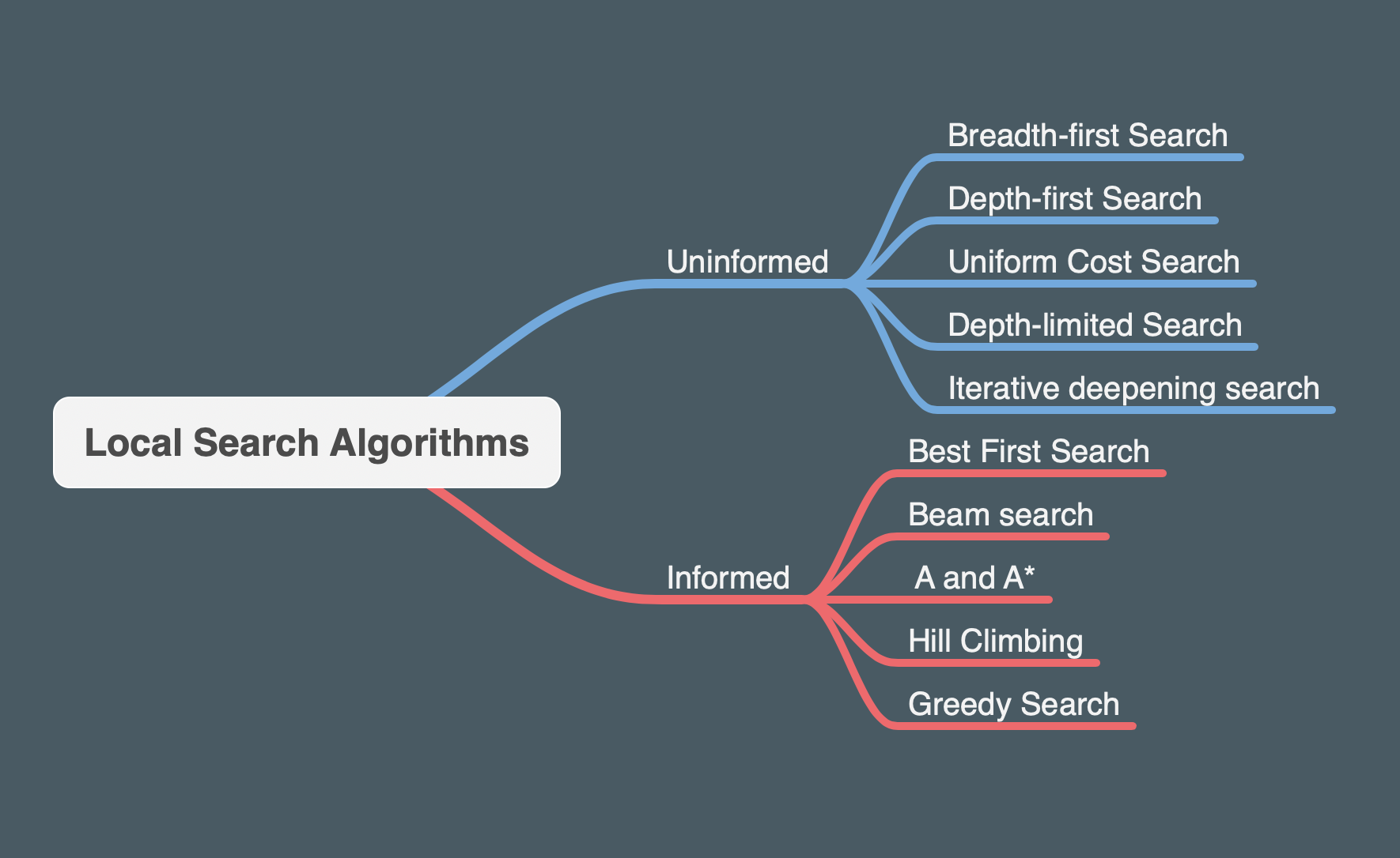The first part of the course teaches us how to formulate a problem (define state space, initial state, goal state, set of actions, and costs for actions). If we can define a finite state space and transitions between different states, this becomes a path-finding problem.

We could use local search methods to look for actions that will lead us to the optimal state.

We first learned different ‘uninformed searches’ such as BFS (will find optimal solution if edges have equal cost), DFS, Uniform Cost Search UCS (BFS variation for edges with different costs), Depth limited Search (DFS but is limited to certain depth and the agent will restart with a different path when it reach a leaf), and Iterative deepening Search (it’s like Depth-limited but depth will keep incrementing if no solution found).

We then learned ‘informed search techniques’ where the exploration is now guided with a heuristic function (based on a prior knowledge) that estimates the distance to the goal (e.g. manhattan distance). Some heuristics are better than others and we generally want it to be admissable (never overstimates) but not to underestimate too much. Some of informed search includes beam search (BFS but explores only the best x edges), A* (like UCS but evaluate each path with heuristic+cost, with the extra condition that heuristic is admissable), and hill climbing (like greedy search but no backtracking).

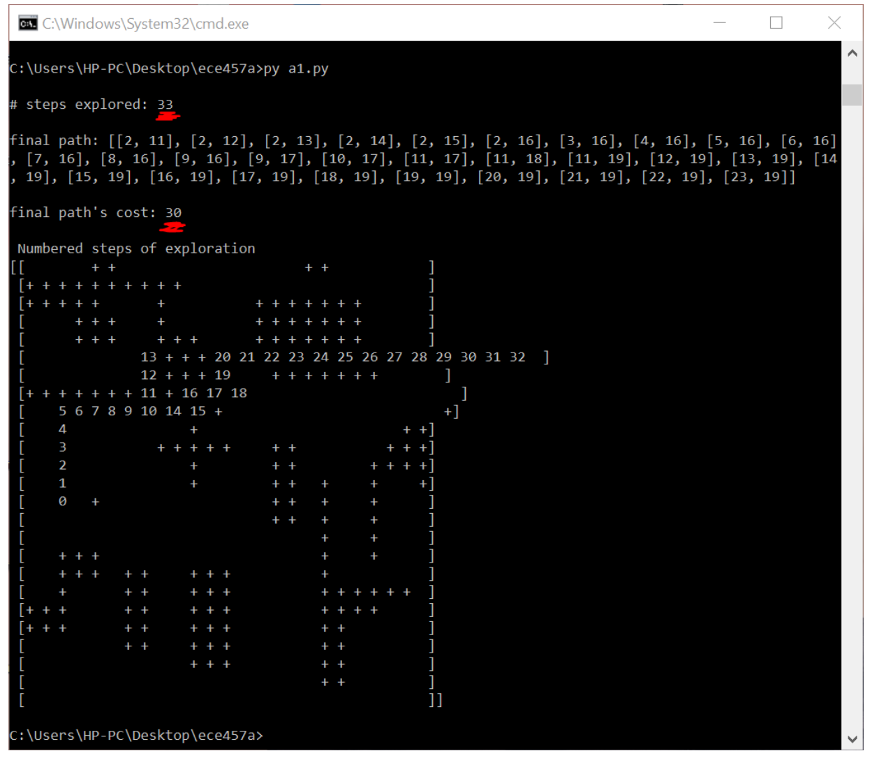
Assignment 1 requires us to write some of these algorithms from scratch to solve a given problem. For example, exploring a maze. The image below is an example of an output of my maze search using A*. It finds an optimal path after exploring 33 states.

B) Game Playing

We then extended the search to the field of Game Playing, where the goal is not just to find a goal state, but is to respond and beat an opponent. There are many complex game types, but we only learned Min-max 🔽🔼 strategy which is only useful for games where we have perfect information. The idea is to pre-generate a tree to look ahead certain steps. One agent tries to maximize some utility, while another tries to minimize. After generating the tree, the computer simply plays them and take best value each turn. The utility is dependant on the game (e.g. in tic-tac-toe, it could be # of open row/col/diag for you - # of open row/col/diag for yout ooponent).

In addition we can optimize min-max using ‘a-b pruning’ 🍇 algorithm that can minimize the size of tree generated by ignoring bad moves that the opponent won’t likely take. The logic is pretty 5head. When generating the tree using DFS, if we think the oponent won’t choose a path because it has found a better one, then we don’t even have to generate more nodes for that path.

In the assignment, we created an intelligent computer agent that plays the game of Conga. Since the states for this game are much larger than tic-tac-toe, the agent only looks 3 moves ahead, generates a tree using min-max with a-b pruning.

C) Meta Heuristic

With informed search algorithms we introduced heuristics. These are good for simple state space, but in more complex ones, it gets you to a local minima. With meta-heuristics now you’re introduced with the idea of exploring vs exploiting, where sometimes you take risks (non-improving actions) and look at the big picture. There are a couple of techniques we covered which is classified as trajectory method (train one solution at a time) and population based (train multiple solutions at once)

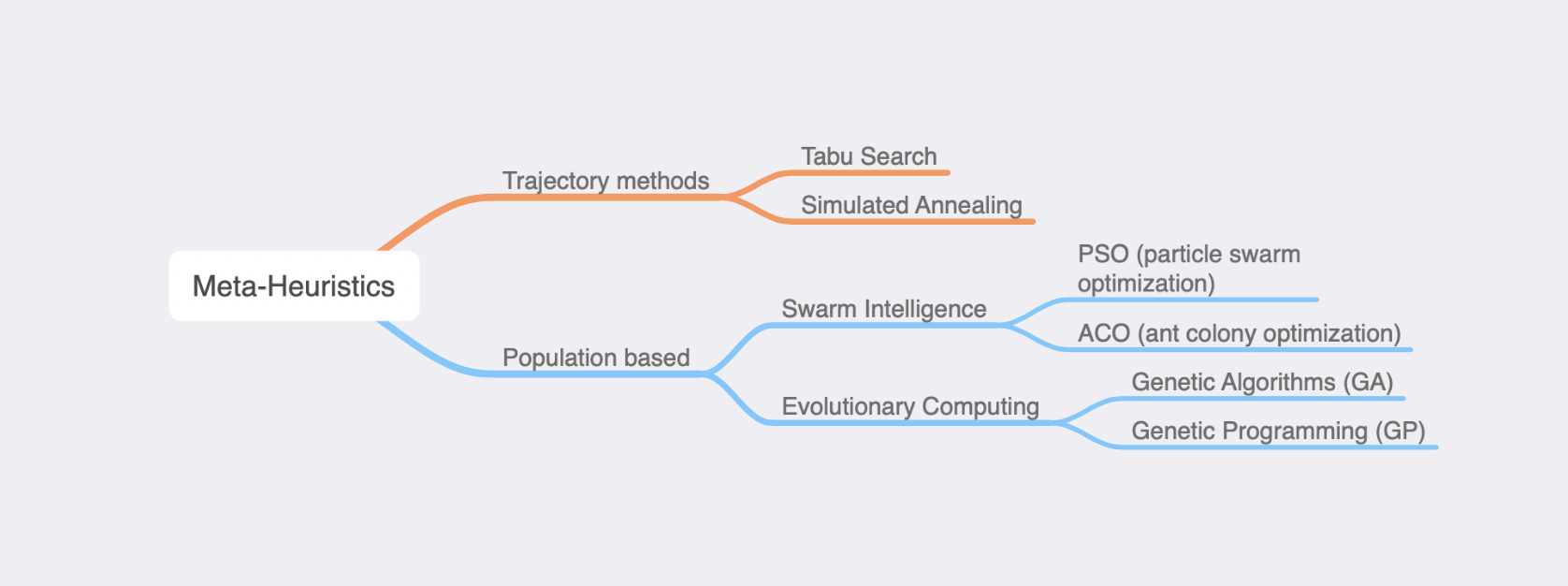
Overall this part of the lecture seems to me like many different approaches to essentially the same problem. In the assignments we get hands on to building these algorithms from scratch which was valuable, but they are all similar problems.

For example in the trajectory method assignment, we were asked to implement Simulated Annealing ♨️ to solve global minimum of a function, solve VPR (vehicle routing problem), or use tabu search 🚧 to optimize QAP (quadratic assignment problem). Generally it’s a matter of first representing the solution (permutation or vector), then defining actions that take you to neighboring states (e.g. swapping 2 elements in the permutation), objective function (to calculate the cost of a solution), and finally use some logic for the agent as it recursively explores/optimize its neighbors. In simulated annealing, the idea of temperature simply motivate the search to explore in the beginning and slowly exploit over time. Tabu Search on the other hand promotes exploration by introducing the idea of short-term and long-term memory so we can avoid visiting the recently-visited or most-frequent solutions.

With the same goal in mind, we also learned population based techniques like PSO, ACO, and GA. These are systems inspired by nature (but generally solves the same optimization problem). For example, in the assignment we used genetic algorithm GA 🧬 to find optimal solution for PID controller parameters, ant collony (ACO) 🐜🐜 to optimize a solution for travelling salesman problem, and particle swarm (PSO) 🐟🐟 to solve for a minimum in a multivariable function. The general idea is to first encode a population of random initial solutions - In PSO we refer to it as a swarm, in ACO it’s a colony, and in GA we refer to solutions as chromosomes. Then it will do certain operations/behaviors to bring that group of solutions to optimal. - In GA 🧬, we mimic the evolutionary process where we select individual chromosomes to a mating pool, mate them together through crossover and mutations to create new offsprings which then replaces the old generation. Over time the population will improve since chromosomes with better fitness (evaluated with some objective function) tend to survive and reproduce. - In swarm intelligence , we mimic the a group of agents that communicate with each other to survive. For ACO 🐜🐜, these are ants. Each ant in the colony communicates with other ants by giving out pheromone given a good path. This is an indirect communication, and we would store these pheromones for each path/state. There are many ways an ant transition between states (transition rule), update its pheromones (e.g. online/offline update), and how the pheromones evaporate. Over time we expect the colony to choose path/transitions that lead to best fitness. - In PSO 🐟🐟, we mimic agent that move in synchrony (e.g. bird’s V formation, fish swarm, etc). We encode each solution as a particle in the search space. Each particle/solution in the swarm holds its own position, velocity, etc. And at every step in time, each agent moves with some inertia (random exploration), tendency to move to its personal best, and tendency to move to its neighboring agent’s best (exploitation). Thus given a topology, neighboring particles will share information and over time the entire swarm moves and converge towards the best solution.

Its a short summary, but there is so much research in each of those areas. It’s often a problem of understanding the tradeoff when choosing the value of control parameters, choosing the right representation for the solution, fitness function, choosing different methods to mutate/crossover/recombine solutions in GA, different methods to update pheromones and transition in ACO, and velocity update rule in PSO. A huge chunk of this course was also plotting performance and testing out different parameters ourselves. Clearly it is a trial/error process ⚖ to choose good parameters and is often problem-specific. Since the course is about cooperation/adaptation, there are also some introduction to how these parameters could ‘adapt’. For example in GA we could include the control parameters as part of the solution representation. This way the controls will change over time with the solution.

D) Genetic Programming

This is pretty dope. It’s like GA 🧬, but we use those concepts to construct programs (AST) 📜 and optimize it to perform certain functions. Thus lets say we have a black-box system where we can observe its response to inputs. We could generate a program (consisting of operations and terminals) that would mimic that system.

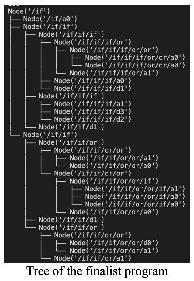
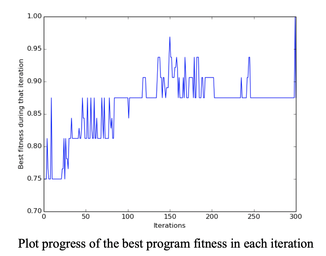
For example, in the assignment we create a python program that construct other programs (AST) 📜 that would mimic the behavior of a 6-mux, using binary operators AND, OR, NOT, IF. We evaluate the fitness of a solution (AST) by feeding it inputs and getting % of correct outputs. Like GA, a high-fitness solution will tend to survive. The following shows the final 6-mux my program generated, as well as the progress of the population fitness over 300 iterations:

We then covered a bit on evolutionary programming (although there wasn’t assignments on it) where instead of evolving programs, we evolve machines (FSM). Generally it could be used to build machines that recognize and classifies patterns.

E) Reinforcement Learning

We then jumped into a brief discussion of RL 🕹. A newer class of AI. This was mostly review for me since I’m also taking ECE 493 this term

F) Thoughts

All in all, I love how this course is very hands on. Some of the assignments really took quite long because we have to code everything from scratch. Primarily for the GP and Conga game-playing assignment it took a really long time to code the environment (although the logic was pretty straight forward). But at the end of the day, it was fun and rewarding.

A wide range of topics was covered, and definitely clears up a lot of my misconceptions about AI systems. The strategies learned in this course is definitely useful for lots of things like optimizing a function, optimizing weights for a neural network, clustering objects to optimize certain fitness, scheduling time-tables given certain soft/hard constraints, etc. Maybe I’d find myself a hard problem to solve in the future and play with these algorithms a bit more.

2. Reinforcement Learning - ECE 493

493 are special topics in ECE which offers different topics every year. This year it was RL and so it does feel like the course outline is still under-developed since its their first time teaching it. Well, added with the unexpected event of online classes, it wasn’t anyone’s fault. Some assignments got extended and others cancelled. However, I think it was complete enough for me to explore further on my own in the future.

The idea of RL is simply to learn based on experience, normally without prior knowledge. When the agent interacts with the environment and performs an action, it will transition to another state. At the same time it recieves a reward for that move. We generally try to simplify the problem into an MDP model which means the next state depends only on the current state and action.

Some important concepts was the idea of ‘policy’, ‘value-function’, and ‘action-value-function’. The policy is simply a function that maps a state to the probability of taking each action. We try to optimize for this policy. For example, given we’re in a state, one optimal policy might direct the agent to move right. Value-function V(s) is a function that maps a state with a value indicating its expected return from that state. Action-value function Q(s,a) is a function that maps a state and an action to the expected return. Overtime as the agent repeatedly take actions and get rewards🍰/penalties🥊, it will eventually learn the environment and seek the long-term rewards 🏆.

A) K-armed Bandit

The course first introduced the simple stationary scenario of a K-armed bandit. We have k slot machines 🎰🎰 and the agent had to pull a lever each iteration. These levers are biased around an expected mean. So an agent would have to repeated test all levers to determine the optimal lever that gives highest reward. But how long should it explore before it is sure that a lever is worth exploiting? A lever could potentially appear to give good rewards but in the long-run there is something better. So there are different approaches to balancing exploration/exploitation such as epsilon-greedy based on an incremental average reward, UCB selection, thompson sampling, etc.

B) Dynamic Programming methods

We then learned concepts of MDP model, epsiodic/continuing tasks, returns, discounting rewards, and Bellman equations which offers a recursive property to update the value-function. This leads to Dynamic Programming RL approach - which repeatedly execute policy evaluation (improve value-function based on policy) and policy improvement (translate the new value-function into our new policy) until it converge to our optimal policy. Two variants of the DP algorithm is ‘Policy Iteration’ and ‘Value Iteration’. The main disadvantage of this is that it assumes the agent knows the environment dynamics (agent have perfect knowledge of how the environment will react with the next state and the reward, given an action and current state). This is often not the case in real life.

C) Monte-Carlo methods (TD, multi-step bootstapping)

We then moved to monte-carlo methods, where the agent samples a complete episode from the environment, before updating its value function with bellman equation. Unlike DP it learns only based on experience. It will converge given that every state-action pair is visited. We also make distinction between on-policy (perform backup based on the agent’s actions) and off-policy (perform backup based on other actions) variations.

Then we get into TD algorithms. While DP 🏟 goes wide, and Monte-carlo 🎢 goes deep into the search space, TD(0) 🐾 only samples one step ahead. We generally use prediction error and use its difference to update our model. Two variation of TD is SARS'A’ and Q-LEARNING. SARSA is on-policy (update backup based on next-state S’ and next action A’), while Q-LEARNING is off-policy (backup is based on max return. It learn one thing and does another). We learned that Q-learning tend to take more risk and although fast/better in practice it doesn’t guarantee convergence. But recently people come back to it because of neural-network and DQN. A variation of SARSA and Q-Learning is Expected SARSA and Double Q-learning. These 2 algorithms is simply a variation to try and minimize sample bias 👨‍🦯 (by being more observant).

From TD(0) we could generalize the equation for multi-step bootstrapping algorithms TD(λ), where λ is the number of steps to sample. Previously SARSA and Q-learning is TD(0). But with λ > 0, we could accelerate learning as rewards get spread faster instead of updating a step at a time. The natural method would be forward view where we store rewards and go back in time to update the discrete steps you took. This is usually inefficient, and there is an equivallent backward view where we introduce ‘eligibility trace’ 👣👣 which stores a decaying count for each state that increments when you visit that state. Thus, this tracks the most recent steps and enables us to distribute the rewards to previous steps without storing each of their returns.

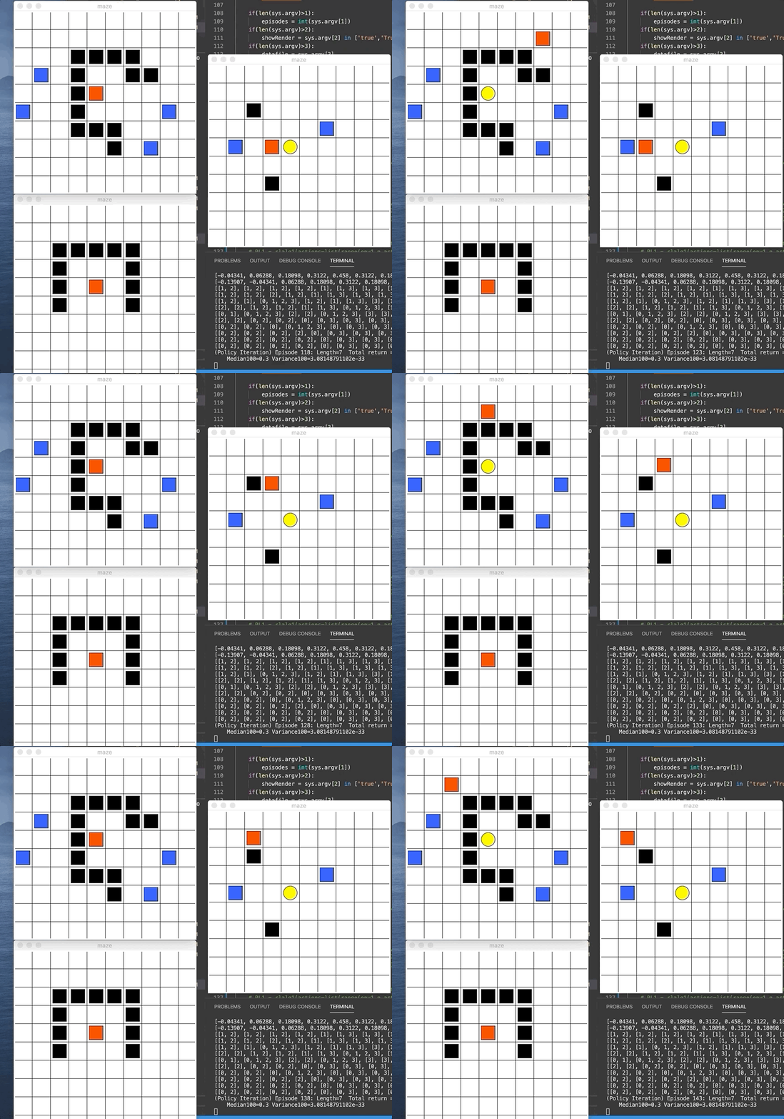
We did 2 assignments where we get to code those algorithms hands-on for a given MazeWorld environment. I got to implement policy iteration, value iteration, Q-Learning, SARSA, Expected SARSA, Double Q-Learning, and SARSA with eligibility trace. For each, we plot the performance over iterations and compare its behavior. The gif below demonstrates the red agent 🟥 as it learned the goal 🟨 (reward +1) and avoid the blue pits 🟦(penalty of -10) and black walls ⬛️. We give each step a penalty of -0.1 so the agent naturally try to find shortest path.

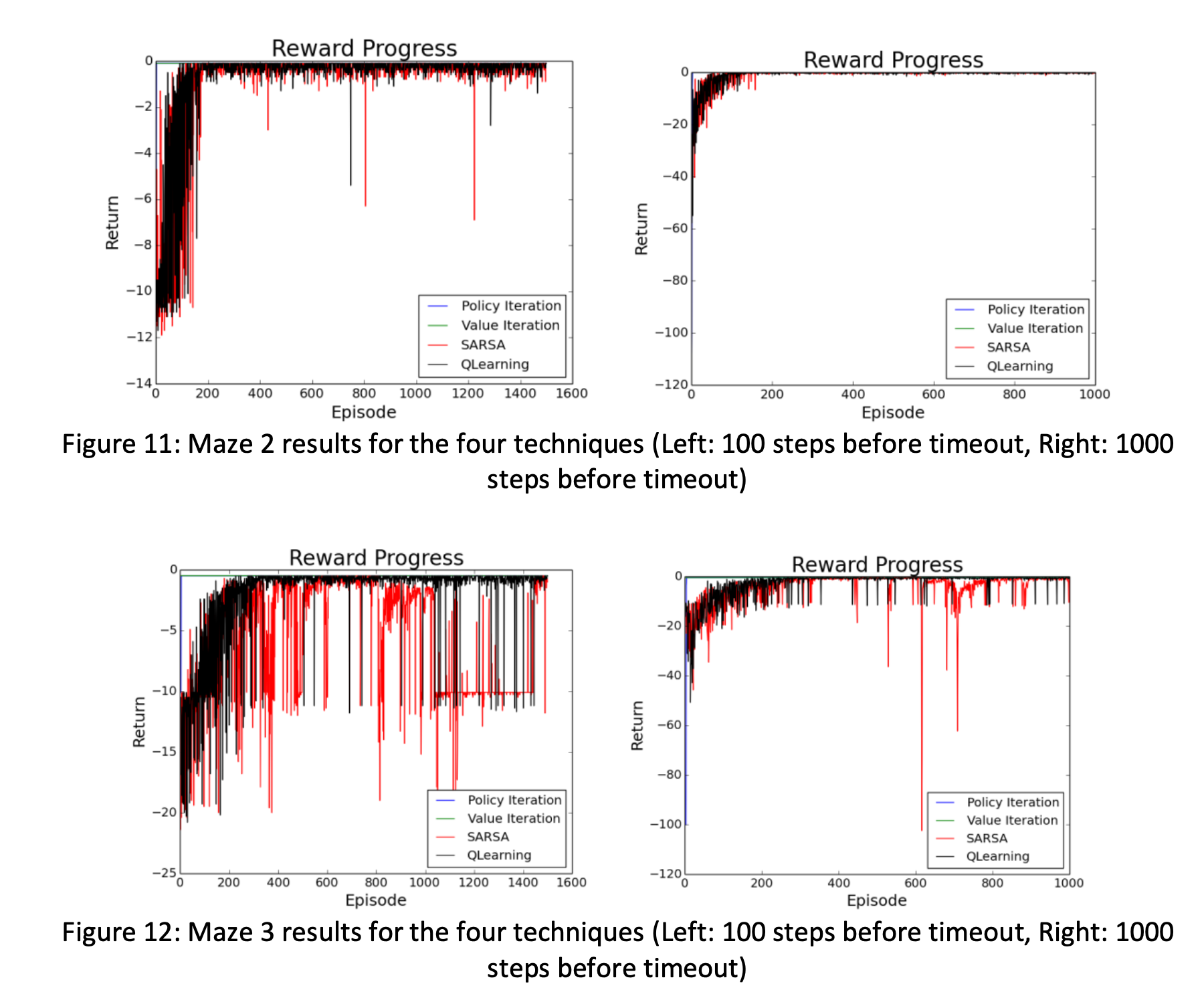
As shown in the sample performance graph below, DP algorithms like value-iteration and policy-iteration converges really quickly (but assumes that we know the environment perfectly). While the SARSA and Q-learning will continuously sample and take hundreds of iteration before finally converging to a stable value.

D) Policy Gradient

We then learned policy gradient. This is where we optimize the policy directly without maintaining a value-function. One advantage is that it can learn continuous actions. It also reduce overall memory since we’re no longer keeping a table of value-function in cases where states are huge. In fact, we generlaly use a stochastic policy where instead of a table mapping state to certain actions, we could use softmax function (for discrete action space) or gaussian functions (for continuous action space). We then use the gradient update rule (derived from SGD) to update the weights. These weights are used to approximate the value function for us. Value function approximation could be done by a number of ways such as linear function approximation, coarse coding, tile coding, etc. These value function approximation are just different ways to encode the state and action space.

In assignment 3 where we had to implement a policy gradient with the same MazeWorld environment as before. I represented the states-action pair with 1-hot encoding as a 1x400 vector (the first 100 entries indicates moving left from each of the 100 states in the grid, the second 100 entries indicate moving right, etc). With a simple linear function approximation and softmax function for the policy, I didn’t see my agent converging at all 😢 even after 5000 episodes (which took like 30 minutes to run).

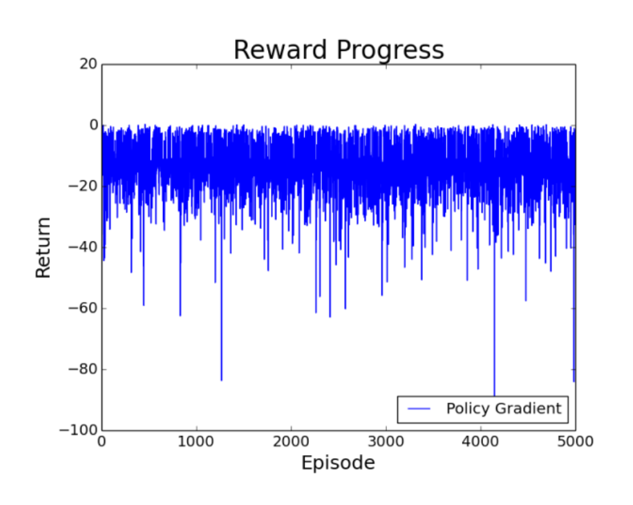
Maybe a potential improvement would be to try other ways to represent the features or incorporate more information like how far the agent has gone from a wall, etc. Instead of doing linear function approximation and softmax function, a better alternative in terms of performance would just be to use non-linear approximations such as using a neural network to learn the policy. But I didn’t really know how neural network works (this wasn’t taught to us) and how to use tensorflow/pytorch libraries - maybe will look at it myself in the near future.

E) Thoughts

RL was a interesting area indeed and the course was an excellent 💯 introduction. There is a good book available online, which is popularly referenced by many RL sources and used in this course. I begin to read it until Monte-Carlo chapter and stopped because of the load of deadlines to catch up this term. But I’ll maybe consider reading it the next few weeks after I’m done with 4A.

The prof also refers us to Spinning up for DeepRL by Open AI which is a good learning platform that extends from things we learned in this course. I’m really excited to check that out too.

All in all, RL is just a lot of Math 🧮. It’s relatively new branch of AI and I think would be exciting to follow.

3. Distributed System - ECE 454

A) Initial motivation

My previous internships were mostly web-related. The most recent one at Loblaw Digital, I realize that maintaining an widely used service is not trivial at all. We deal with distributing our load across multiple nodes, measuring metrics like throughput and availability, building microservices that internally communicates with each other, etc. Nonetheless I think this course was extremely relevant to my field of work so far and useful in the future.

The course was so heavy with information. So I will proabably just try to outline the broad topics such that I would come back to my notes when I need them.

B) Architectures

We learned different styles of architectures to constitute how distributed components interact. - layered 🍔(involve calls between layers. More latency but is scalable and higher throughput). - layers are mapped to physical tiers (machines). A logical layer could be distributed vertically (seperated by physical tiers) and horizontally (split across machines. e.g. db sharding) - Object-based (components are split by objects. Not limited to communication between adjacent layers. But is limited by the vendor - e.g. JavaEJB) - Data-centered (app share it’s state through DB) - Event-based (components react to events like pub-sub)

Normally, it is a combination of different architectural types. We went over a few case study of how peer-to-peer works (communicate without server in an efficient way using an overlay network), Bittorrent (combine p2p + client-server), and self-managing systems (feedback and make adjustments to parameters).

C) Services and Microservices

A service is an encapsualted reusable component. An service-oriented architecture (SOA) is an architecture where services are maintained independently. Interaction can resemble the architectures in (B). Microservices-based architectures is a more loosely defined SOA, where data is not shared and don’t rely on routing middlewares (more scalable and fault tolerant but need coordination).

We introduce web protocols that allow inter-service communications, like SOAP (XML-based) and REST (stateless interaction)

D) Processes + Networking Basics

We went over inter-process communication which was a revision of ECE 354 (OS course), and basic networking which was a revision of ECE 358 (networks coure). IPC is expensive due to context switching while threads communicating within the same process is easily done through shared memory. The OS can support multi-threading using ‘LWP processes’ and/or follow a dispatcher/worker design to dispatch work to threads from the network. In terms of virtualization, a distributed system normally runs in JRE (we isolate app from OS to solve portability) or VMM (portion of server, including OS, is rented out in commodity computing). Server clusters is normally 3-tiered (client load balancer -> app servers cluster -> DB).

A big chunk of the network review was implementing built-in Java client/server sockets, and parameters to control the inter-process communication between server-client.

It’s then followed by Assignment 0 where we implement a server code that opens socket and accept connection one client at a time to process some work until the client closes connection.

E) Communication & Apache Thrift & RPC Performance

Then we covered the higher-level abstractions for inter-process communication protocols. The methods discussed was RPC (2-way comunication) and Message queuing (1-way communication). We learned they’re differences in terms of referential and temporal coupling. Calling an RPC is simply like calling a function in the perspective of the client code. RPC framework like Thrift offers a middleware that generates the client/server stubs for us (to send/recieve message) and does all the marshalling. Thrift also requires both client/server to adhere to a single file defining the communication interface (written in IDL). RPC could be synchronous/asynchronous.

One big question I had would be how I’d prefer RPC over REST. It seems like there’s a lot of debate on this (e.g. performance vs simplicty) and after much googling and watching a debate of gRPC vs REST, at the end of the day it just depends on the use case. They solve the same problem. I’ve never worked with gRPC but it seems like it supports streaming and client can subscribe to responses asynchronously 😳.

Anyway, in Assignment 1 we get our hands dirty with Apache Thrift, in order to build a scalable distributed system where we have arbitrary client nodes, a master server node (FE), and a bunch of worker nodes (BE). FE and BE nodes does the same operation. The system should be fault tolerant towards BE failures (if the worker crashes or spawn new nodes, FE should identify it and move on without failing client requests). I remember this assignment being super hard because we need to recognize how to keep track of the BE nodes asynchronously, how to handle RPC communications, etc. There are many kinds of server implementations in Thrift like TSimpleServer, TNonBlockingServer, TThreadpoolServer, etc, and they have their own tradeoffs. I feel like thrift documentation was REALLY bad though (not sure if you’d even call it one).

We also learned how to calculate RPC performance theoretically, and determining if our throughput is client-limited or server-limited. It was useful in the assignment since we could calculate our throughput (based on number of request, round-trip time) and compare that against max throughput (depends on server threads and calibrated time spent to perform single request).

F) Distributed File System & HDFS

Moving on from communication protocols, we now focus on applications of Distributed system. One of it being DFS. We covered a case study of 2 popular DFS systems.

First is NFS, where client use RPC to remotely request for files in the server. There are many variations and features in NFS like client-side caching, upload/download model (as opposed to remote access model), different semantics of file sharing (how replicated files can behave), and how one server can export/mount a sub-directory of another servers’ files.

The second case study was on GFS (HDFS is open-source version of this). When large data are distributed across servers (or striped). The client would request the master (store cache and update logs) for the address of the chunk it’s looking for, then directly pull data from the chunk server. There is also protocol to update files in all GFS server replicas.

G) Hadoop Map Reduce & Apache Spark & Pregel

The idea of map-reduce is to scale a computation (ideally small computation but large data). There are many working nodes where each node takes am input file from HDFS, split records (key-value), randomly put it in the mappers, The mapper does some operation and spits out >= 1 key-value pairs, then a partitioner shuffles that output across nodes (across network), and feed it to a reducer (sorted based on key such that key-[list of values]). The reducer than aggregates it and emit an output record. There is fault-tolerance built in Hadoop.

We then learned Apache Spark, which could do the same thing as Hadoop MR but leverage the use of RDD (a distributed in-memory). Spark has transformation (output an RDD) and action operators (output scalar).

Another distributed computing framework but specific for distributed graph processing is Google’s Pregel. It partitions the vertexes from large graph where each vertex has its states, and could distribute information/computations each iteration (supersteps). This could be used for things like Pagerank and finding shortest path.

In assignment 2, we perform different analytical computations of a large data set using a Hadoop solution and a Spark (written in Scala) solution. It was pretty simple and was overall truly impressed by the speed that it performs to analyze a really HUGE dataset.

H) Consistency and Replication

Moving on to learning about consistency of replicated data stores, we learned some theoretical consistency models (defines how much data is allowed to disagree on a state), like Sequential consistency, causal consistency, linearizabiity consistency (strongest), and eventual consistency. We then discussed impementation to maintain these models such as primary-based protocols (similar to Assignment 3), quorum-based protocols, and how to achieve eventual-consistent replication where we use Merkle tree to exchange data between replicas.

Tbh, this part of the course got me super confused 😨. I get the theory, but when it comes to having to debug the code for linearizability in the assignments, I was so confused 🏳. It was probably the hardest assignment of the course in my opinion. In assignment 3, the goal was to implement a distributed key-value service; using Thrift to distribute the key-value pairs, and Zookeeper to coordinate ZNodes between the servers to determine which server is primary and all others would be replica. We got the basic function eventually but there would be small scenarios like when primary server shutting down and restarting very quickly before the Znode got deleted (so it would see itself as a primary which is invalid, the client would send get/put request to that invalid primary’s address which leads to linearizability errors, etc.). Anyways I kinda gave up on trying to debug the linearizability errors in the end, but the assignment still helps me have a better understanding of Apache Zookeeper’s role for service discovery and nodes to store coordination data.

I) Fault Tolerance & Consensus problem & RAFT & Distributed Transaction & Checkpoint Recovery

We begin by clarifying what it means and the metric used to measure availability, reliability, safety, and maintainability.

We’re first introduced to the ‘consensus problem’ (coordination problem, where processes vote to reach a consensus). Depending on whether the processes are sync/async, or message sent have to be in-order/out-of-order, or communication delay is bounded or not, or if it’s unicast/multi-cast, there are certain mixture of these cases in which a distributed consensus is possible. This is a real limitation, and is ‘solved’ in practice using frameworks like RAFT. RAFT works by a distributed log (storing the commands to execute) which executes locally to replicate a state machine. RAFT select leaders, replicate the logs, and allow consistency.

Aside from consensus, we talk about ways to ‘detect failure’ in RPC calls. When server can print its log before/after operation, what are some strategies server could use to print logs such that client could identify when crash occurs. The moral of the story was that no matter what reissue strategy client uses (e.g. client resends request on failure), or error-logging ordering strategy server uses, you cannot get exactly one type of semantics. We just choose the semantic that leads to best for our use-case.

Another problem of fault tolerance is to execute a ‘commit transaction’. One solution is using two-phase commit (2PC) for distributed atomic transaction, where like the consensus problem a coordinator make sure every server is ready to commit (through a voting process), before making a global commit. If one participant fails, the entire commit is aborted.

Another problem of fault tolerance is recovery with a ‘distributed checkpoint’. There’s an algorithm to ensure all process temporarily halts to take local checkpoints (such that its then possible to take a recovery line and recover the entire distributed system from that point onwards).

J) Apache Kafka

Apache Kafka has a couple of APIs like producer/consumer (simpe push/query topics), connector API (for data from DB), and stream processing (which combines producer/consumer with more powerful features). Interesting usage could be messaging between apps, activity tracking, collecting metric and logs from different systems, real-time count, etc. Topics could be partitioned further (but we only did single partion in A4), and operations could be done for specified window and hop size.

In assignment 4, we used the Kafka Streams API to take the streams from 2 topics, perform some operations and provide the output on 1 output topic. In the end we have a program that alerts the output topic in real-time when classrooms are over-capacity. Kafka does fault tolerance by default so it wasn’t as hard, and now I think I have better understanding of manipulation/conversion between different stream types like KStream -> KGroupedStream -> KTable, etc. Stateful operations like reduce/aggregate allow us to compare new state with previous state. A challenge I faced was the case when a studentA moves to a new classroom. Upon this even, we had to decrement the occupancy in studentA’s previous room. Turns out if our count is stored in a table, KTable and KGroupedTable could solve that automatically since the key-value could be something like studentId:roomId.

K) Clocks and CAP Principle

I realize I took for granted that computer clocks are synchronized where in fact it is hard to do so. Clocks diverge for many reasons (like relativistic time dilation, network delay, different tick rates at different temperatures, etc). One way to resolve this is using NTP protocol using something like a client/server protocol where computers refer to one another and adjust they’re clocks to a reference clock (lower stratum). PTP provides better accuracy but NTP is still more widely used.

Alternatively, without trying to synchronize clocks we could still agree to event orders using Lamport clock (ensuring time is consistent with happens-before relation during communication, where reciepient of message will adjust its clock - a incrementing scalar), or Vector clock (Like lamport but now each process stores a vector of the clocks for all other processes).

The CAP principle claims that you can’t get consistency, availability and partion tolerance at the same time (you can only have 2). So in distributed system when you have a partition (network failure and nodes can’t communicate), you can either choose to prioritize consistency (e.g. banking transaction) or availability/latency (e.g. shopping-cart, social applications). In other cases you might make this tunable (tunable consistency) where you have quorums and the size of R/W quorum is the parameter you control to tune the level of consistency/availability tradeoff. One example is Apache Cassandra which is quorum-based key-value store and support tunable consistency.

L) Thoughts

Distributed System is hard 🥵. The course helps us scratch the surface of it so if I come across it one day I might understand some concepts. But it really introduces us to the reality of almost all modern systems today. In reality, life is just not perfect, there are more than one way to do things, and there are tradeoffs that had to be made for pretty much everything.

There is a textbook for this course which I probably won’t bother reading. I feel like these are things I’d dive in once again when I see them in future projects/problems, which I’m sure I will.

4. Robot Dynamics and Control - ECE 486

No offense but this was proabbly the hardest course I’ve ever took in my entire life. At some point in the course I kind of lost hope but was so greatfull to have a lab partner that didn’t. She would motivate me to work it out together, which things actually did in the end 👏. First of all, I acknowledge that robotics is cool but I didn’t know what it really is before this course. We learned controls in ECE 380 and probably around 2 other courses before that (about root locus, PID controller, etc). So I was pretty excited on further learning about it and how it’s practically used.

Because it was online our prof decided to have a ‘new way of teaching’ where there are no lectures, and he have us independently read textbook on Perusall (a social e-reader where we can ask questions by highlighting texts). The online classes would then be used for discussions about any questions we have and solving quiz solutions. More than 50% of the class dropped out in the first 2 weeks (and part of me regret that I didn’t). We had a reading + quiz every week and project + lab bi-weekly. I spend more time on this course than other courses I had this term. But tbh at least for me, I’m not sure how rewarding that grind was. The textbook was “Modern Robotics: Mechanics, Planning, and Control” and the author includes youtube videos for every topic. The topics were super math and physics intensive. Crunching lots of matrices 😬yikes forever.

Project

The Project (individual) are done in Matlab Grader, where the core goal is to build a ping-pong robot simulator. The project is divided into sections distributed across the entire course where we get to apply the topics learned. So from the beginning, we generate the trajectory of the ball given initial velocity, then get the T matrix of the desired contact position if we’re given the position of the ball, design the robot (with joints and links), plot and identify singularities, calculate the inverse kinematics analytically (given desired contact position, find the joint angles to achieve it), then generate a joint trajectory (that moves the paddle from home position to its contact position) within certain duration and ensuring it stays within the joint limits, then define the dynamics of the robot (mass matrices and rotational inertias - essentially assigning them masses that properly satisfies movement of the robot in response to external force like gravity). Finally, I try to tune the PID controller so the robot follows the trajectory correctly without any steady state errors, overshoots, delay, etc. - Some parts of the project were cool. There was so much struggle to pass the Matlab Grader’s test cases, and I had to redesign the robot a lot of times..

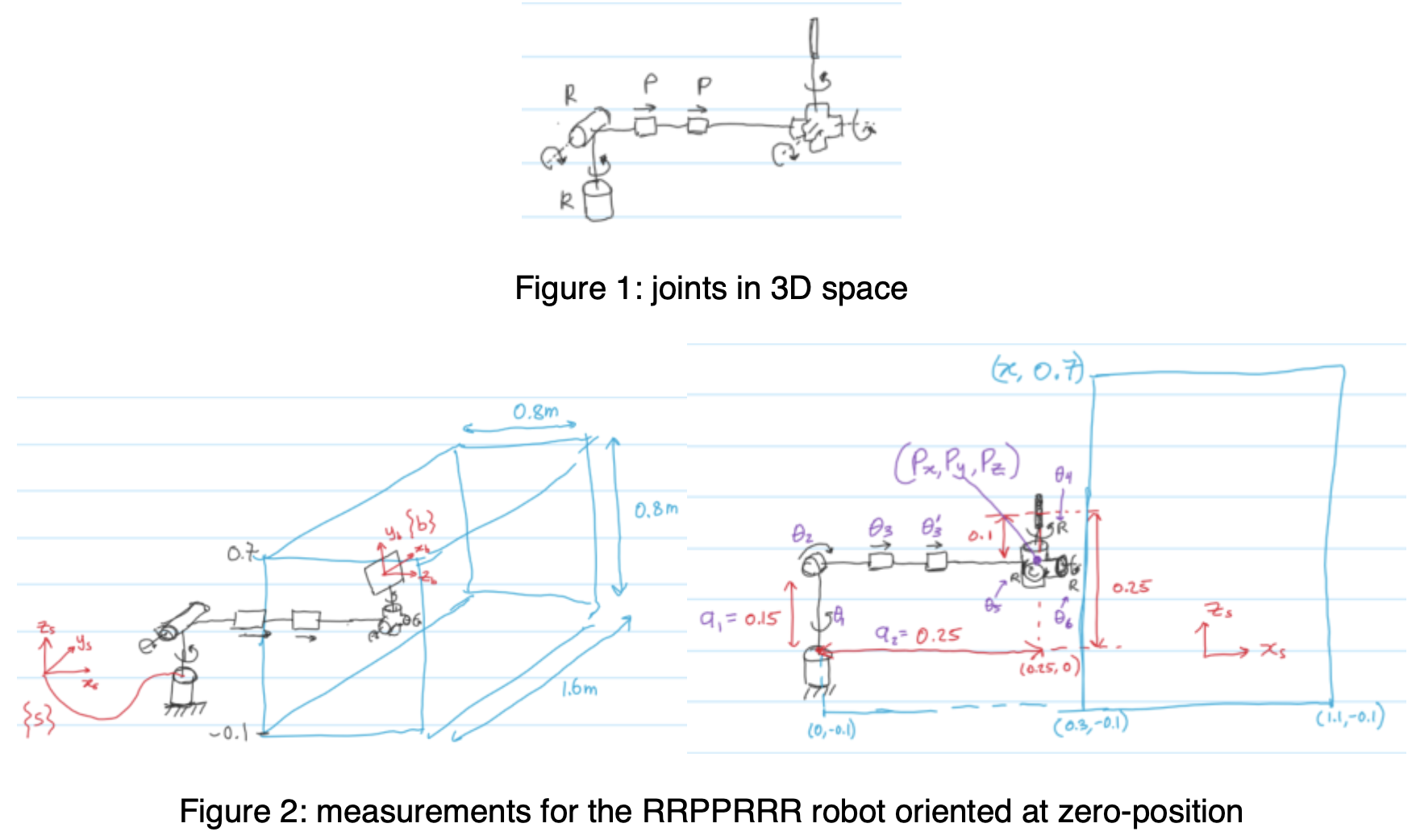
Below are some of my scuffed designs and how it changes over time:

The First Robot I designed..

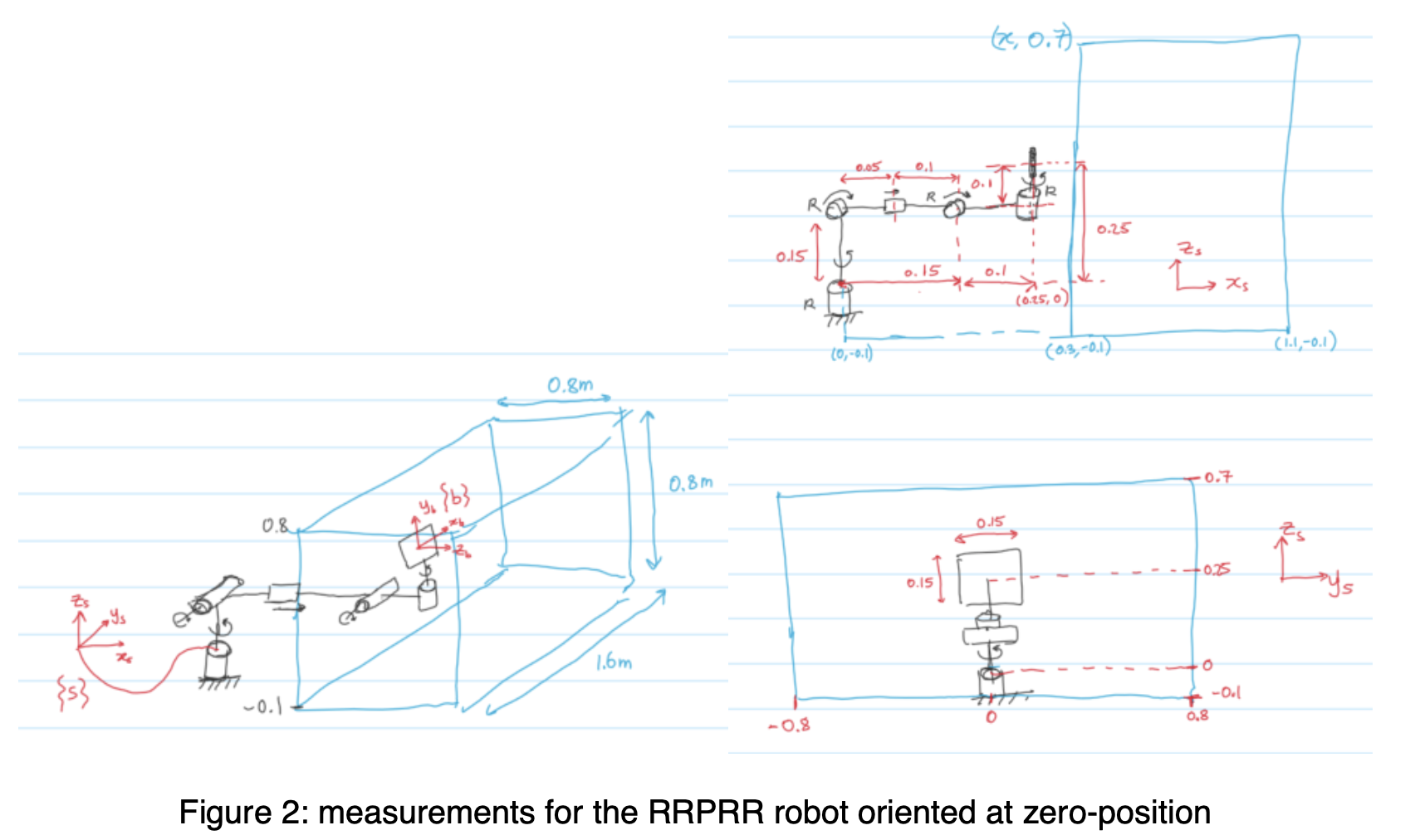
Then trying to get the Inverse Kinematics working, I end up re-deesigning the whole thing..

Then trying to get the Dynamics working so here’s the final redesigned robot. The last joint is prismatic joint that goes up and down with the paddle at the bottom edge of it.

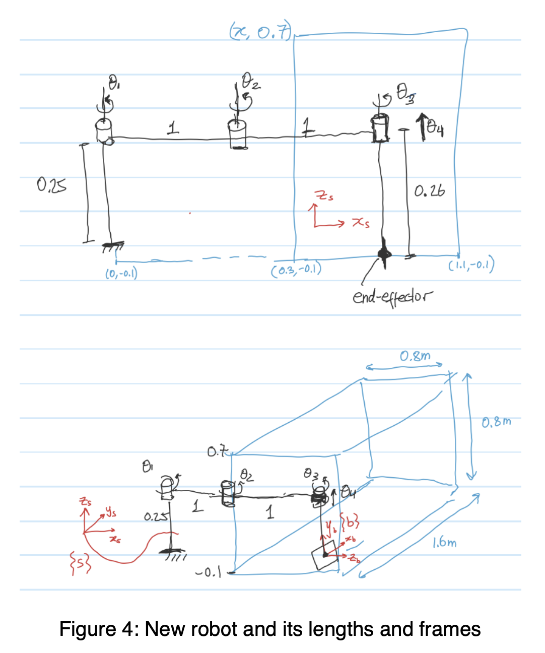
and the design for links and joints of the robot..

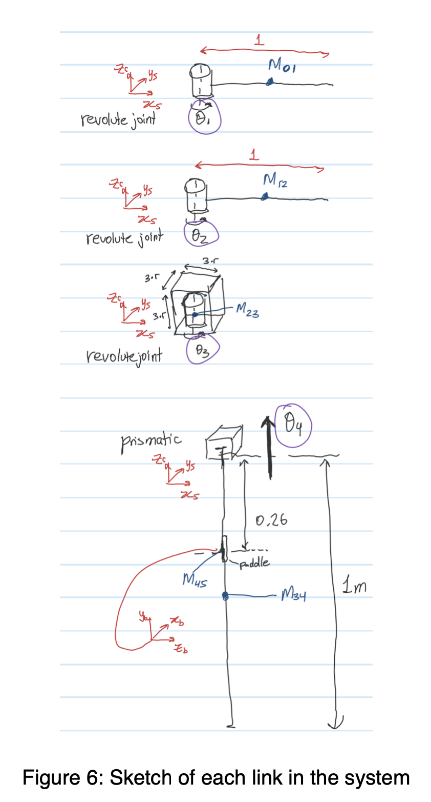
Labs

The Labs (group of 2) are done in Choreographe and we get to control a real NAO robot. Since it’s all online this term, we only see the robot in simulation, while the TA runs our code in the physical robot to give us feedback to reflect upon. Like the project, labs are also seperated into modules throughout the course. For example we perform Forward Kinematics and inverse kinematics on the robot’s right arm, generate a trajectory, and code a controller loop to follow the trajectory. This was equally as difficult as the project but it was cool to see the movements reflect directly on the NAO robot. The TA also gave us a video sometimes (and as shown below, shit happens.. all the time 💩).

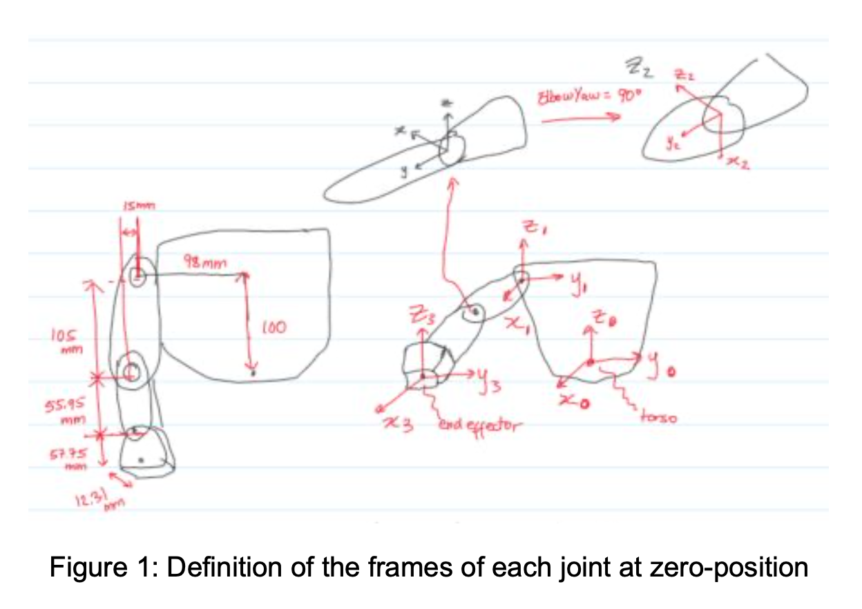
Course Modules

Just summarizing the course topic chapters in my own words:

• Configuration Space:
  • got to know terminologies like Task space, workspace, C-space topology, and how to calculate degrees of freedom (dof). For me it also introduced for the first time different joint types (revolute, prismatic, spherical, etc) and the dof that it allows/constrain.
• Rigid-body motions:
  • lots of new terminologies like rotation matrices SO(3) to rotate with respect to either space/body frame, how to change between reference frames, expressing angular velocity using skew matrices (rotation about some axis), exponential coordinates SO(3) vs matrix logarithm so(3) and formulas to switch between both representations. These are pretty much different ways to represent a coordinate and a rotation (a coordinate is also a rotation about some axis from the space frame).
  • then we get to ‘Transformation matrices T’ SE(3) (4x4 matrix). Unlike rotation matrix (3x3), this now tells the rotation + translation. Similarly we have now ‘twists’ which represents linear + angular velocity (twist can be represented as 6-vector or using a screw representation). We also have an exponential coordinates SE(3) vs matrix logarithm se(3) to represent coordinates. Finally we get introduced to wrenches (a vector consisting of moment + force), which is also measured with respect to some frame of reference.
• Forward Kinematics
  • The position and orientation of the end-effector of a robot can be obtained by FK. The components of FK is the home position of the end-effector M (this is the T matrix for end-effector when all joint angles are 0), then the screws of each joints (for a joint i, the screw is a 1x6 vextor [w1, w2, w3, v1, v2, v3]. w defines the rotation axis and v=wxr where r is a vector from the origin frame {s} to the axis w). With all those components we can plug in the FK equation.
  • The input to FK is arbitrary joint angles and it outputs the resulting end-effector position and orientation.
  • You can represent FK in terms of space frame, body frame, or do a D-H representation (which simply define a T matrix from each joint to the next and multiply them together)
• Velocity Kinematics
  • Jacobian matrix - can be used to convert rotational speed of the joints into velocity of the end-effector of the robot. It could also be used to convert from joint torques into forces of the end-effector at the tip.
    • Jacobian matrix can be calculated column-by-column manually (screw axis all relative to {s}. We did this in the quiz and labs), or use adjoint of matrix exponentials which could be harder to do by hand.
  • Learned about singularity, and how it’s represented in a manipulability and force ellipsoid. At singularity positions, the tip can’t generate velocity/forces in a particular directions (e.g. of singularity is a straight arm). As we move closer to a singular position it’s normally harder to move.
    • The ellipsoids tell us the direction that end-effector move with least effort vs greatest effort
• Inverse Kinematics
  • Reverse of FK. Now given the desired final end-effector position, we use IK to generate the angles of each joint. (there are many solutions. e.g. lefty-righty and elbow-up-elbow-down solutions)
  • To find IK, we could do it analytically or numerically. We did analytical in the project, quizzes, and labs which was so painful (a bunch of pure vanilla geometry to compute the angles given end-effector position). The numerical is an approximation method using Newton Raphson method over iterations - normally we compute analytical IK and feed it to the software to make it more accurate.
• Trajectory Generation
  • trajectory is made up of ‘path’ (a series of robot’s position over time) and a ‘time scaling’ (defines the progress of the path. Take values [0,T]).
    • trajectory could be in joint space (list of desired joint angles) or task space (list of position matrices)
  • We covered point-to-point trajectories (from one point and stop at another) and via-point trajectories (where goal is to pass through series of via-points at specific times).
  • There are different time scaling types like cubic or 5th-order polynomial, trapezoidal motion profiles, and S-curve time scaling. This choice basically controls how smooth we want the robot to be (e.g. we might not want infinite ‘jerk’ 🤡 - a sudden change in acceleration)
  • In the code library we used for the project, there’s a function to generate the trajectory for us, given a start and end position and the choice of time scaling.
• Dynamics of Open Chains
  • Forward Dynamic - goal is to find joint acceleration given the joint angle, velocity, and torque.
  • Inverse Dynamic - goal is to find torque given joint accelerations, force, joint angle and velocity.
  • The 2 ways to do this is by Lagrangian Dynamics formulation (so much MATH. We define the object’s inertia matrix and mass matrix by defining its center of mass) or Newton-Euler formulation (a recursive algorithm)
  • The math starts to overload in this chapter and I just stop understanding…
• Robot Controls
  • We review about P, PD, PID controllers, and how the equation converts to error-dynamics of the controller (e.g. damping, stability, steady-state error, overshoots, etc.)
  • Learn general structure of using feedback from the actuator and sensors to the controller so it computes the error and send a new controlling signal to the actuators.
  • Again, I stopped understanding and pretty much gave up on project portion of this chapter where we had to adjust Kp, Ki, Kd controller to achieve smooth tracking.

Dear Future Steven.

Do you still find the above explanations/concepts unclear? Same. I hope you’d get it someday though. If not that’s alright. At least, I hope reading it reminds you once more of your darkest moments in life..

No words could describe how much stress this course put me under. Not only is the materials difficult, but it’s just a constant struggle to understand things due to a lack of in-person support. Despite that, I do gain much more respect for robotics, and I do find the IK and FK portion to be super POG. I think I definitely feel more confident with Matlab after the course.

5. Psychology - Psych 101

Oh Yes! Psychology! My favorite course this term!

I’m really glad I took this course. A lot of reading but here and there I’d see eye-opening theories that helps me understand myself as a human a bit better 👽. A good break from all the technical courses too. The course has greater than 5x the gloasary of concepts compared to ECE 454 so I definitely won’t go over everything.

But what I’ll do is go over maybe 1 or 2 fun facts from each chapter/module. (I actually lied, I can’t resist putting more fun facts. Bear 🐻 with me)

1. Memory
   • May seem counter-intuitive, but our least accurate memories are those we think about the most (since it’s reconstructed each time it’s used, errors are introduced each time)
   • Children are prone to leading questions. You can easily create false memories in children. Thus we should avoid interrogation techniques when interviewing these little creatures 👶.
   • With classical conditioning, you can associate a neutral stimuli with significant event, so the next time you introduce the cue/stumli it will trigger automatic action. (e.g. bell + dog = drooling, after being paired with food)
2. Stats and Research Designs
3. Evolution and Psychology
   • Evolutionary psychology studies problems that occur in ancestral environment that could affect our mental adaptations. (E.g. humans is naturally better at some problems involving survival in ancestral past)
   • Parental Investment theory: Male and female (of a given species) have different degree of obligation to invest in offspring. In species where fertilization occurs in female (ie. humans), the male tends to be more competitive and female tends to be selective when choosing a mate. (explains why I’m single)

4. Perception

   • ‘Perception’ is the process of giving sensory input a meaning.
     • some people with ‘Synesthesia’ have condition where their sensory stimuli crossover between different modals (eg. they taste something when seeing a color, Grapheme-Color synesthesia, etc)
   • ‘additive mixing’ 🌈 of light (when we mix lights, they’re wavelength adds) vs ‘subtractive mixing’ 🎨 of paint (red objects absorb light of all wavelengths except certain ranges which it reflects as red. When we combine red with green paint it absorbs even more wider range of wavelengths and those that don’t get absorbed is reflected to us as color brown). This was mindblowing because I never realized the distinction between mixing colors for light vs pigments. For computers which emits light, the RGB system is an additive process (colors adds up to white). In the contrary, if you are a painter, you care more about subtractive mixing of colors (colors adds up to black).
   • We percieve depth in 2 ways.
     • Binocular cues: 👀 Our 2 eyes allow left/right eyes to figure out discrepancies, and that degree of disparity indicate distance. Closer object have higher disparity.
     • Monocular cues: 👁 These cues includes Interposition, Linear Perspective, Relative Size, Texture Gradient, Visual Acuity, Motion Parallax (here’s a cool art based on motion parallax - far objects move slower), etc. These make really cool optical illusions and art that tricks us into percieving distance.
       • With such intricacies I was curious how depth perception could be implemented in AI. Seems like last year Google AI had successfully learned depth perception using ~2000 Mannequin Challange videos to Supervise the learning. Since only the camera is moving they could get accurate depth maps of the scene and use that huge data for training the model. 🤩
   • Although our hearing is 360°, our auditory acuity is poorer at locating objects in space (unlike bats). We locate objects through hearing using 2 techniques
     • ‘interaural time differences (ITD)’: 🦻 the delay / time difference between reaching left and right ear (sensitive to low frequency <1.5kHz which is dominant in everyday sounds)
     • ‘interaural level differences (ILD)’: 🎧 our head casts an acoustic shadow going to each ear. So its louder in one ear than the other. (more effective for high frequencies)
     • CASA (computational auditory scene analysis) ☕️ is a field that study how we can decompose the complex waveforms of different sources and locate them. (uses could be smart hearing aids, cochlear implants, speech recognition, etc.). After googling things, it looks like ‘source separation’ had been studied for decades now. But look how cool it is (HARK, an open source robot audition software). March this year, Facebook also released Demucs, a music source seperation system with AI.
   • Our brain can stop pain if it needs to (Aron Ralston amputate himself from a rock. ‘descending pain modulation system’ is activated when survival > pain)
   • Endorphin cause an analgesic effect (helps you endure pain). Social reward (like holding hands, being present for others) have pain-reducing effects too. In contrary, negative emotion and attention to pain can increase sensitization to pain (distraction is common technique used in hospitals. But social support and emotional factors give a more long-term treatment for chronic pain)

5. Consciousness

   • There are many theories on why we dream 😪 with supporting reasons and also critics. E.g. Wish fullfillment, Problem Solving (Help us discover creative solutions), Mental Housekeeping (allow brain to strengthen connections with learning and memory), or Activation synthesis (claims that dreams are just accident because of the neuronal activity in brain during REM sleep) are some of these theories.
   • Almost all mammals have rem sleep. But we’re not sure if animals have cognitive capacity to construct narratives 🐖
   • Hypnosis is just heightened state of suggestibility. Things like making you stronger, recovering lost memories, are all myths. But it’s true that it has anesthetic affects (inhibits pain), and is a good way to insert false memories.

6. Problem Solving

   • Under threatening conditions, people raised in lower social-economic status tend to prefer immediate rewards, while people wth high SES tend to conserve what they have and wait expecting a better future.
   • When information is incomplete (informal reasoning), we rely on 2 types of heuristics
     • ‘Available heuristic’ (based on what comes to mind first)
     • and ‘Representative heuristic’ (based on how closely it resembles your expectation. (e.g. guess based on stereotypes)
   • When communicating, the speakers/listeners share a set of knowledge (common ground) that evolves at every exchange
   • Primates with larger brains 🧠 (humans) tend to live in larger groups (e.g. human can maintain ~150 relationships)
   • Linguistic labelling (putting things in words) alter neural process. When having negative thoughts a part of the brain is activated less when they’re not given the chance to label things. So writing/talking about negative emotions will actually improve your well being, but keeping it to yourself is bad. (people should talk about their problems 🗣).

7. Emotion

   • ‘Cognitive appraisal’ (how you explain events) affects emotion. (e.g. if you think someone bumps into you on purpose you will feel mad vs if you appraise the situation as being an accident then you’re less angry)
   • Theory of mind (cognitive development) only begins to develop at 3. (Infants have no cognitive capacity to feel guilt and shame)
   • Unlike emotions which can be negative/positive, ‘drive’ has no valence. It’s always beneficial for survival. Drive state always tries to maintain an ideal level (homeostasis). (E.g. Hungry/full and sexual arousal)

8. Development 🤰

   • In embryotic stage, mistakes can happen during cell division that cause birth defects. So the purpose of miscarriage (by evolution) is to terminate pregnancy early and restart to eliminate waste of resource.
   • There’re many threats to embryo/fetus development (e.g. maternal nutrition, drug use, illness, teratogens)
     • HIV: Since blood supplies are seperated by placenta membrane, HIV don’t get transmitted to the baby. However the virus can still be transmitted during birth when there’s blood contact.
     • Teratogens are carcinogenic/mutagenic chemicals in food that’s harmless to us but pose threat to the embryo. (coffee, animal products, etc). Too much at certain development stage can lead to miscarriage. By evolution, morning sickness and food aversion are adaptive solutions so pregnant humans avoid these foods.
   • First 6-8 months, an infant don’t have preference over caretaker. After that period they begin to develop attachment with primary caretaker and have stranger anxiety.
   • Mary Ainsworth’s experiment shows different child-parent attachment styles. 👩‍👦👩‍👧
     • Secure attachment (healthy bond) - Explore confidently when mom is present, protest when mom leaves and calm when she returns
       • occurs when mom is sensitive and attentive (child knows that she will notice and be in position to act when they’re in danger)
       • lots of things affect this ‘attentiveness’ (e.g. martial satisfaction, infant’s temperament, socio-cultural factors, etc)
     • Anxious Ambivalent attachment (non-secure) - Explore anxiously when mom is present, protest when mom leaves, difficult to console after her return
     • Avoidant attachment (non-secure) - Infant unconcerned about mother’s presence, don’t protest and don’t greet her when she’s back

9. Freudian and Humanist Theory

   • Freud theory of personality - claims that our personality is an interaction between Id (pleasure seeking), Ego (rational and realistic), and super-ego (moral component and guilt). This is like PIXAR movie ‘Inside Out’
     • when unconscious thoughts are full, threatening urges begin to bubble up to the conscious and this becomes ‘anxiety’
     • Defence mechanisms to anxiety could be repression, projection (misattributee thoughts), displacement (redirect impulses to another), regression (immature patterns to avoid adult problems), rationalization (invent faulty excuse to justify themselves), etc.
   • Carl Jung propose that goal of life/development is to strive for superiority (refers to improving one-self). E.g. children study to compensate our inferiority and adjust ourself to adults.
   • Carl Rogers propose that everyone have a ‘self-concept’ (mental representation of who we are, qualities, typical behaviors). When we choose action we invoke this self-concept (e.g. “what would a person like me do in this situation?”). But when we see incongruence (disparity between our self-concept and reality), we tend to distort reality to fool ourselves (e.g. blaming)
     • Rogers believe incongruence happens when you believe love is conditional 👩‍❤️‍👨. If you believe in unconditional love (others love you despite your actions), then there’s little motivation to hide yourself.
     • incongruence lead to anxiety. Anxiety motivate self-deception. Which leads to greater incongruence, … (endless loop). ➰
     • Moral: believe that people will love you for who you are. Then maybe you’ll have less anxiety.

10. Behavior in Group

    • Bystander Effect - responsibility is diffused/spread across number of bystanders. The more people there are, the less likely someone will take an action.
    • Social Loafing - (for cooperative tasks) the larger the group, the lower the effort invested by the members. Countermeasures could be to make individual contribution observable, emphasize task importance, group cohesion (members who like and respect each other are less likely to loaf), specialization, etc.
    • Social Facilitation - (for competitive tasks) If the task is difficult/unfamiliar, the presence of others can hinder/lower your performance. But if the task is easy/well-practiced, then having audience will improve performance.
    • human sort themselves into in-group and out-group. We favor similar people (even in small ways possible, like people who likes the same music as you). In-group members are expected to cooperate. One can work with out-group members well given a common goal (but given a limited resource, conflict may arise).
    • Conformity happens because we don’t want to be an out-group. But when someone else contradicts the group, the pressure to conform may evaporate.
    • Obedience: Milgram experiment shows 50% participants obey to deliver harm to others given an authority figure. Those who are obedient believe they have no choice and blames the authority.
      • Moral lesson: Do the right thing! Believe you always have a choice and should take responsibility in whatever you do
    • Planning fallacy - our tendency to underestimate time to complete a task. (E.g. We tend to leave things to last minute. In a way planning fallacy is also good since it allows us to pursue ambitious projects)
      • I’m guilty for this a lot 😩
    • Persuasion techniques. My favorite is ‘A door in the face’ technique, where you start with a huge request you expect to get rejected, then compromise after.
    • In 20th century, there are more ambiguous biases (people don’t openly express prejudice). E.g. aversive racism where one feels unconfortable and find excuse to avoid certain situations. The reaction will be ambiguous to both parties and hard to interpret.
      • hopefully in 21st century we start to recognize each other by our character instead of the cover.

11. Depression Anxiety and Schizophrenia

    • How we treat mental disorders depends on the model we use
      • Medical model: we diagnose and try to find a cure (some criticism of this model involves issues of over-prescription, ‘is it a disease vs behavior’ argument - e.g. homosexual used to be treated as a mental disorder)
      • Supersticious model: In the past, people drill holes in the head because they believe its demonic posession. Or killing witches if it was believed to be a result of witchcraft. 🧙‍♀️
    • Sometimes anxiety and low moods are important psychological process. Supressing them with drugs may cause more problems than it being a solution.

12. Psychological Therapy

    • Freud used to do psychoanalysis to uncover unresolved conflicts that hides in the unconscious. Methods include dream analysis and free association.
      • e.g. “Tell me more about x.”, “You didn’t mention about this, why is that?”
    • Carl Roger propose ‘client-centered therapy’. He believe anxiety comes from incongruences between reality and our self-concept. The cure is to promote belief of unconditional love 👩‍❤️‍👨.
      • Therapist is just there for clarification, and to show empathy and genuineness. We call ‘clients’ not patients since therapist-client share equal status and responsibility in this therapy.
    • Cognitive Threapy instead tries to reorganize habit/thought patterns.
      • e.g. “Let’s see what happens when you actually fail. It’s not the end of the world…”
    • Behavioral Therapy tries to solve problematic behavior using conditioning. (believe that the root problem is irrelevant. The problem is in the behavior)
      • e.g. exposure therapy, aversion therapy, etc.
    • When stressed, and the event is controllable (e.g. exams), ‘problem-focused coping’ like working harder and planning better is effective. But under uncontrollable events (e.g. death of someone) ‘emotion-focused coping’ like watch movies and relax would be the better strategy.
    • Maintaining different social roles (e.g. you could simultaneously fulfill your role as a father, student, coworker, basketball team member, etc) is good for your health. More encouragement around you.

6. Capstone Design Project - ECE 498A

Nothing much to say about this course. It’s just a bunch of report-making. A huge deliverable we had was finishing up the design for our Fourth Year Design Project (will be due next year around April). Our project is about tech for mental-health which we’ll see in the future 😋. A highlight from this course was having to schedule interviews with lots of mental health experts on UW campus to understand the problem.

7. What’s next?

TBH I need a break. (We have 3-4 weeks vacation! 🏖). Someone suggested on the class Slack channel that the goal after finals is not to crash. Since we have been in a heightened state all term, a sudden crash has a high chance of making us stuck (whatever that means). So we were suggested to plan something to do after finals as a way to “train down” the mind.

For me, writing this blogpost was part of it. I’ll also try cooking bunch of stuff and nurture my Ukulele skilz. Definitely should get more sleep. My local rock climbing gym is also open now. There’s also a couple of books I’m looking forward to read.

Oh and after lots of interviews this term, I luckily got a intern position for next term (September till December) at StackAdapt as a Software Developer (I’m guessing full-stack but we’ll see where they put me). I think I’ll be wfh from Waterloo since the office is in Toronto. It’ll be interesting to have a wfh internship all term 😳… Super pumped up tho! It’ll be my 6th and last coop/work term.